Manipulating images can be an essential task in data science as it allows for data augmentation which can improve data accuracy by reducing overfitting. In this post, I walk through how to manipulate images using only numpy!
First thing to do is import the necessary packages:
import numpy as np
from skimage import io
import matplotlib.pyplot as plt
numpy will be used to manipulate the image while skimage loads and saves the image. matplotlib will be used to display the image after making changes.
After loading these packages, let’s load in our image:
camaro = io.imread('camaro.jpg')
print(camaro)

>>> [[[ 83  81  43]
  [ 57  54  19]
  [ 34  31   0]
  ...
  [179 144 112]
  [179 144 114]
  [179 144 114]]

 [[ 95  93  55]
  [ 72  69  34]
  [ 46  43   8]
  ...
  [181 146 114]
  [181 146 116]
  [182 147 117]]

 [[101  99  61]
  [ 88  85  50]
  [ 67  63  28]
  ...
  [184 149 117]
  [184 149 117]
  [184 149 119]]

 ...

 [[ 12  10  11]
  [ 12  10  11]
  [ 12  10  11]
  ...
  [ 28  27  25]
  [ 27  26  24]
  [ 27  26  24]]

 [[ 12  10  11]
  [ 12  10  11]
  [ 11   9  10]
  ...
  [ 28  27  25]
  [ 27  26  24]
  [ 27  26  24]]

 [[ 13  11  12]
  [ 12  10  11]
  [ 10   8   9]
  ...
  [ 28  27  25]
  [ 27  26  24]
  [ 26  25  23]]]
Printing our camaro variable shows the numpy array of values for the image. The numbers in these arrays range from 0-255, which represent the intensity of the color. It’s important to note the shape, or dimensions, of this array:
camaro.shape
>>> (1200, 1600, 3)
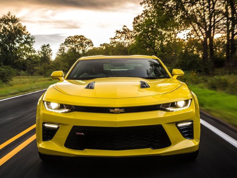
We’re working with an image that’s 1200 px in height and 1600 px in width. The 3 in this tuple is because when the image is loaded, it’s separated into three color channels: red, green, blue (RGB).
Let’s see what image we’re working with:
plt.imshow(camaro)
plt.show()
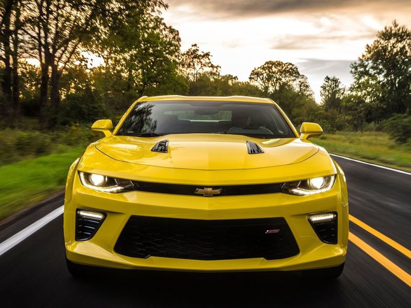
We’ve loaded our image and displayed it using matplotlib! Let’s save this file:
io.imsave('camaro_plt.jpg', camaro)
This code can be used to save any file throughout this walk-through. Alright, let’s see if we can crop this image to just the camaro:
cropped = camaro[350:1100, 200:1400, :]
plt.imshow(cropped)
plt.show()
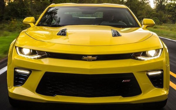
Nice! Using numpy slicing, we’ve selected the values in the arrays to just show the camaro.
Next, let’s flip the image. First, vertically:
vertical_flip = camaro[::-1, :, :]
plt.imshow(vertical_flip)
plt.show()
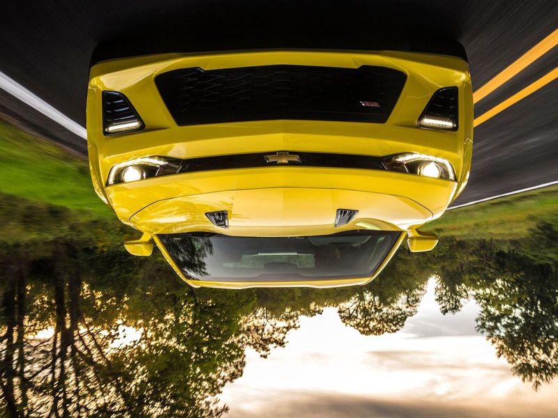
Very cool! We’ve used camaro[::-1, :, :] to flip all values in our first array be selecting the values in reverse order. If we want to flip it horizontally:
horizontal_flip = camaro[:, ::-1, :]
plt.imshow(horizontal_flip)
plt.show()
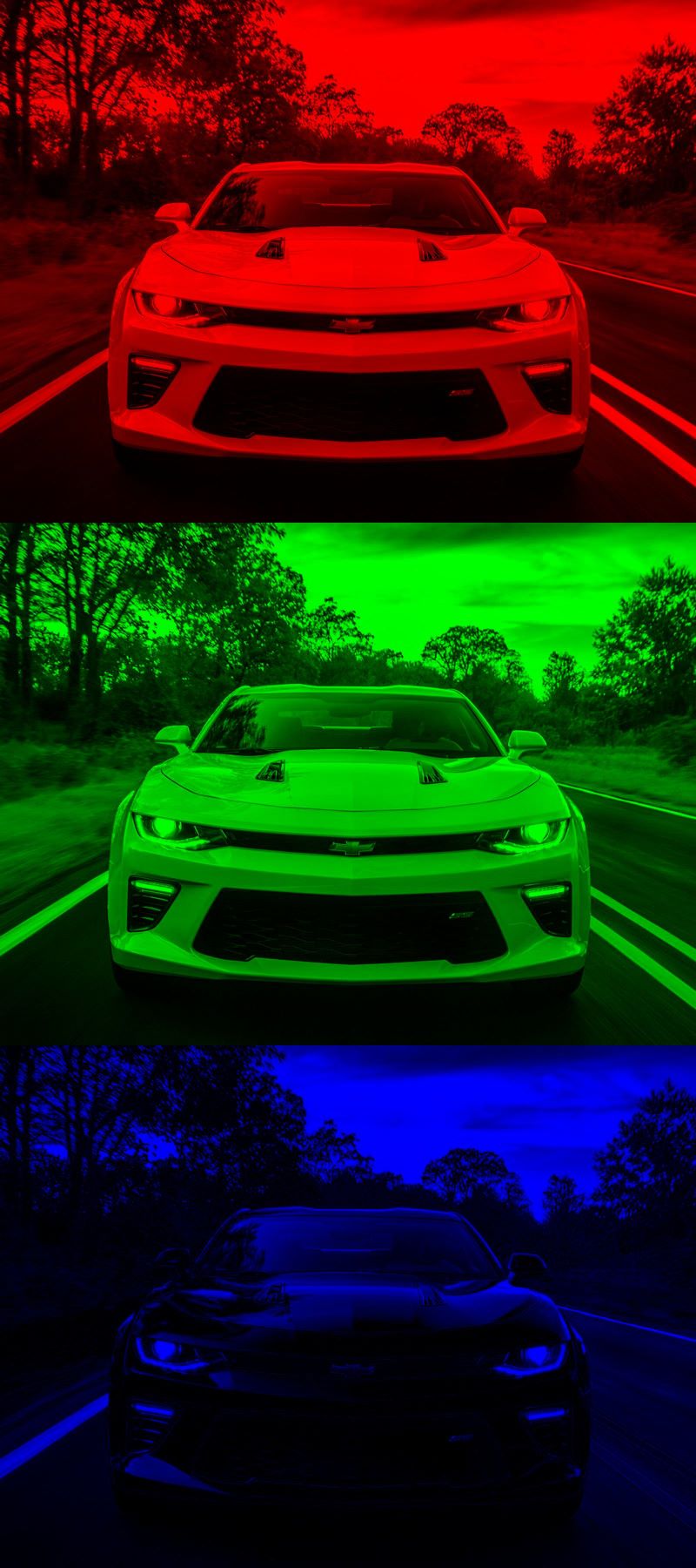
Well done! Now, remember how those three color channels? Let’s have some fun with that. First, lets grab just the red color channel. To do this, we need to zero out the other color channels. If we only cropped out the other channels (selected the red channel only), then our image wouldn’t render as red. To avoid this, we’ll create an array of zeros with the same shape as our camaro array:
red = np.zeros(camaro.shape, dtype='uint8')
Then we’ll set the first array of our red array equal to the values of the first array in our camaro array:
select the first group of arrays
red[:, :, 0] = camaro[:, :, 0]
Let’s see how it looks:
plt.imshow(red)
plt.show()

We can also do this for blue and green:
green = np.zeros(camaro.shape, dtype='uint8')
green[:, :, 1] = camaro[:, :, 1]

blue = np.zeros(camaro.shape, dtype='uint8')
blue[:, :, 2] = camaro[:, :, 2]
Finally, let’s put these together by stacking the arrays:
camaro_rainbow = np.vstack((red, green, blue))
plt.imshow(camaro_rainbow)
plt.show()
